Loading in the Dataset
This code will illustrate the R package (DTVEM) with simulated data available in the DTVEM package.
Click here to download and install the DTVEM package.
First load the DTVEM package.
library(DTVEM)Next load the simulated data included in the DTVEM package, called exampledat1.
data(exampledat1)Get a look at the file structure.
head(exampledat1)## Time X ID
## 1 1 -1.076422 1
## 2 2 -1.904713 1
## 3 3 1.307456 1
## 4 4 NA 1
## 5 5 -4.224493 1
## 6 6 NA 1Illustrating the Inadequacies of the Partial Autocorrelation Function
Next we want to explore lags with typical time series techniques. Run a partial autocorrelation function for the variable for each ID.
#DEFINE THE NUMBER OF UNIQUE IDs
uniqueIDs=unique(exampledat1$ID)
pacfmatrix=matrix(NA,nrow=length(uniqueIDs),ncol=10) #SAVE THE PACF RESULTS FOR THE FIRST 10 lags
#CREATE A FOR LOOP TO RUN OVER EACH ID
for(i in 1:length(uniqueIDs)){
  temporarydata=exampledat1[exampledat1$ID==uniqueIDs[i],] #EXTRACT THE DATA FOR A GIVEN INDIVIDUAL
  pacfout=pacf(temporarydata[,"X"],na.action = na.pass,plot=FALSE) #RUN THE PARTIAL AUTOCORRELATION FUNCTION WITHIN R, IGNORE THE MISSING DATA
  pacfmatrix[i,]=pacfout$acf[1:10]
}
Okay, we have the results, now we have to plot them. Each grey line will represent a PACF estimate for a given individual. The black lines will represent the mean PACF estimate.
plot(1:10,pacfmatrix[1,],xlab="Lag",ylab="PACF Estimate",type="l",col="grey",ylim=c(-1,1))
#FOR EACH UNIQUE ID
for(i in 1:length(uniqueIDs)){
  lines(1:10,pacfmatrix[i,],col="grey")
}
lines(1:10,colMeans(pacfmatrix,na.rm = TRUE)) #PLOT THE AVERAGE LAGGED ESTIMTES
poscrit=2/sqrt(14-1)
negcrit=-2/sqrt(14-1)
lines(1:10,rep(poscrit,10),lty=2) #PLOT POSITIVE CRITICAL VALUE
lines(1:10,rep(negcrit,10),lty=2) #PLOT NEGATIVE CRITICAL VALUE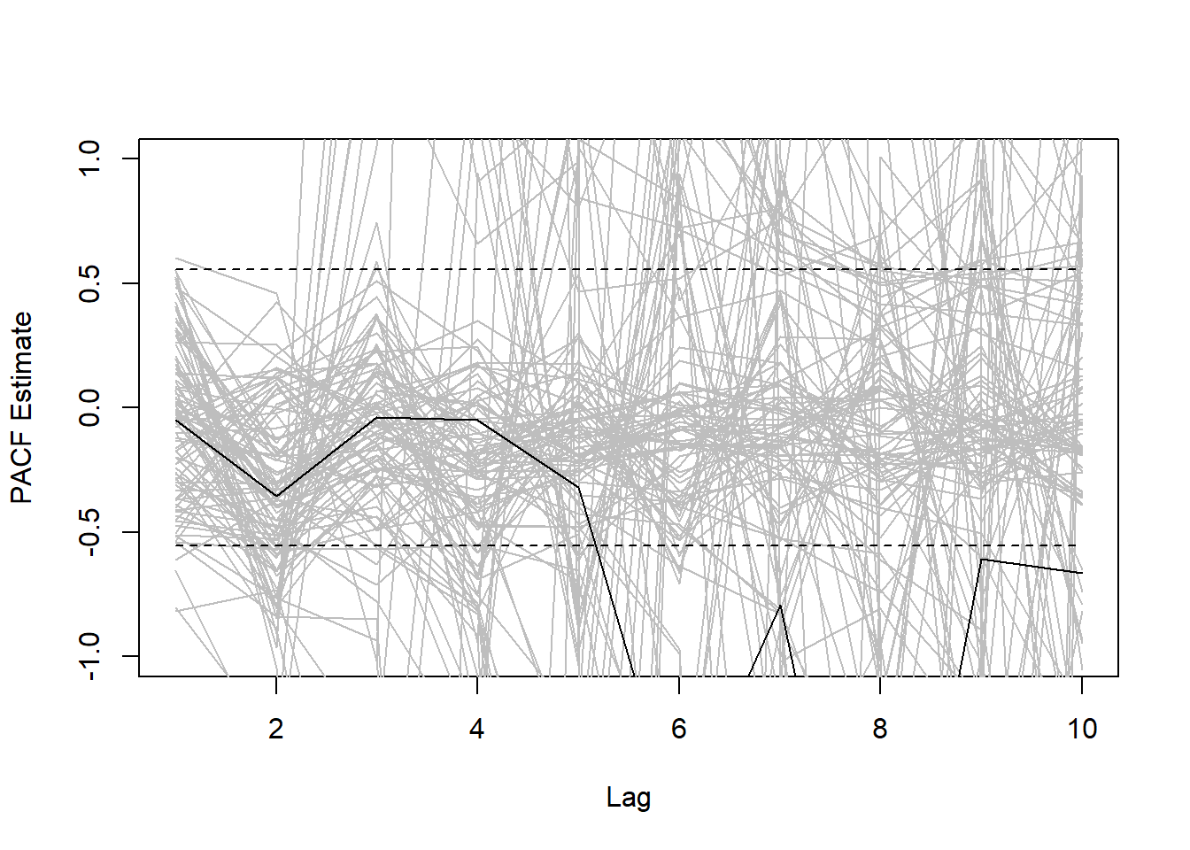
The results look like for any given individual the PACF results are highly unreliable. However, the PACF does suggest that there are potentially significantly negative lags at lag 6, 7, 8, 9, and 10.
Showing the strength of DTVEM
Let’s see what DTVEM has to say about this.
out=LAG("X",differentialtimevaryingpredictors=c("X"),outcome=c("X"),data=exampledat1,ID="ID",Time="Time",k=9,standardized=FALSE,predictionstart = 1,predictionsend = 10,predictionsinterval = 1)## OpenMx version: 2.8.3 [GIT v2.8.3]
## R version: R version 3.4.4 (2018-03-15)
## Platform: x86_64-w64-mingw32
## Default optimiser: CSOLNP
## NPSOL-enabled?: Yes
## OpenMP-enabled?: No## Setting up the data for variable #1 of 1.## Completed stage 1 of DTVEM, now identifying the significant peaks/valleys.
## DTVEM stage 1 identified the following variables as potential peaks or valleys: XlagonXlag1, XlagonXlag2, XlagonXlag3, XlagonXlag4
## Removing group-based time of residuals##
## Begin fit attempt 1 of at maximum 11 tries##
## Lowest minimum so far: 3274.70348452396##
## Solution found##
## Start values from best fit:## 0.225059455018684,-0.237669113091979,0.275143492004439,0.0240822052277956,2.08939869379243## Summary of multisujbject
##
## free parameters:
## name matrix row col Estimate Std.Error A
## 1 XlagonXlag1 s1.A 1 1 0.22505946 0.05061653
## 2 XlagonXlag2 s1.A 1 2 -0.23766911 0.04816207
## 3 XlagonXlag3 s1.A 1 3 0.27514349 0.04666714
## 4 XlagonXlag4 s1.A 1 4 0.02408221 0.05312983
## 5 Xresid s1.Q 1 1 2.08939869 0.10551147
##
## Model Statistics:
## | Parameters | Degrees of Freedom | Fit (-2lnL units)
## Model: 5 895 3274.703
## Saturated: NA NA NA
## Independence: NA NA NA
## Number of observations/statistics: 1400/900
##
## Information Criteria:
## | df Penalty | Parameters Penalty | Sample-Size Adjusted
## AIC: 1484.703 3284.703 NA
## BIC: -3208.880 3310.925 3295.041
## CFI: NA
## TLI: 1 (also known as NNFI)
## RMSEA: 0 [95% CI (NA, NA)]
## Prob(RMSEA <= 0.05): NA
## To get additional fit indices, see help(mxRefModels)
## timestamp: 2018-08-18 10:58:28
## Wall clock time: 7.172824 secs
## optimizer: CSOLNP
## OpenMx version number: 2.8.3
## Need help? See help(mxSummary)
##
## [1] "Variables that should be controlled for are: XlagonXlag1"
## [2] "Variables that should be controlled for are: XlagonXlag2"
## [3] "Variables that should be controlled for are: XlagonXlag3"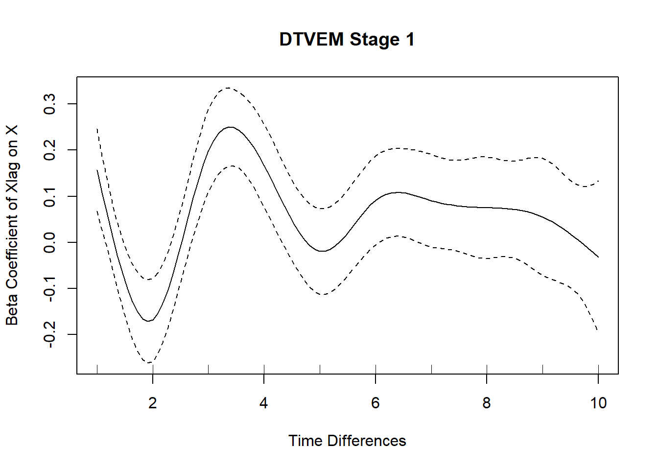
## Completed stage 1 of DTVEM, now identifying the significant peaks/valleys.
## Completed stage 2 of DTVEM (wide format). Now passing to Stage 1.5. Controlling for the following lags in the varying-coefficient model:  XlagonXlag1, XlagonXlag2, XlagonXlag3
## Removing group-based time of residuals##
## Begin fit attempt 1 of at maximum 11 tries##
## Lowest minimum so far: 3274.90917415861##
## Solution found##
## Start values from best fit:## 0.236008799391563,-0.248531920453681,0.2835748499677,2.08271335137451
## Summary of multisujbject
##
## free parameters:
##          name matrix row col   Estimate  Std.Error A
## 1 XlagonXlag1   s1.A   1   1  0.2360088 0.04461888
## 2 XlagonXlag2   s1.A   1   2 -0.2485319 0.04220480
## 3 XlagonXlag3   s1.A   1   3  0.2835748 0.04300307
## 4      Xresid   s1.Q   1   1  2.0827134 0.10448100
##
## Model Statistics:
##                |  Parameters  |  Degrees of Freedom  |  Fit (-2lnL units)
##        Model:              4                    896              3274.909
##    Saturated:             NA                     NA                    NA
## Independence:             NA                     NA                    NA
## Number of observations/statistics: 1400/900
##
## Information Criteria:
##       |  df Penalty  |  Parameters Penalty  |  Sample-Size Adjusted
## AIC:       1482.909               3282.909                       NA
## BIC:      -3215.919               3303.886                  3291.18
## CFI: NA
## TLI: 1   (also known as NNFI)
## RMSEA:  0  [95% CI (NA, NA)]
## Prob(RMSEA <= 0.05): NA
## To get additional fit indices, see help(mxRefModels)
## timestamp: 2018-08-18 10:58:41
## Wall clock time: 9.826756 secs
## optimizer:  CSOLNP
## OpenMx version number: 2.8.3
## Need help?  See help(mxSummary)
##
## [1] "Variables that should be controlled for are: XlagonXlag1"
## [2] "Variables that should be controlled for are: XlagonXlag2"
## [3] "Variables that should be controlled for are: XlagonXlag3"
## This is the #2 out of a possible 10 passes
## Completed loop between 1.5 and 2
## DTVEM analysis completed,congradulations!
## Contact the author - Nick Jacobson: njacobson88@gmail.com if you have any questions.
## Summary of multisujbject
##
## free parameters:
##          name matrix row col   Estimate  Std.Error A
## 1 XlagonXlag1   s1.A   1   1  0.2360088 0.04461888
## 2 XlagonXlag2   s1.A   1   2 -0.2485319 0.04220480
## 3 XlagonXlag3   s1.A   1   3  0.2835748 0.04300307
## 4      Xresid   s1.Q   1   1  2.0827134 0.10448100
##
## Model Statistics:
##                |  Parameters  |  Degrees of Freedom  |  Fit (-2lnL units)
##        Model:              4                    896              3274.909
##    Saturated:             NA                     NA                    NA
## Independence:             NA                     NA                    NA
## Number of observations/statistics: 1400/900
##
## Information Criteria:
##       |  df Penalty  |  Parameters Penalty  |  Sample-Size Adjusted
## AIC:       1482.909               3282.909                       NA
## BIC:      -3215.919               3303.886                  3291.18
## CFI: NA
## TLI: 1   (also known as NNFI)
## RMSEA:  0  [95% CI (NA, NA)]
## Prob(RMSEA <= 0.05): NA
## To get additional fit indices, see help(mxRefModels)
## timestamp: 2018-08-18 10:58:41
## Wall clock time: 9.826756 secs
## optimizer:  CSOLNP
## OpenMx version number: 2.8.3
## Need help?  See help(mxSummary)
##
##          name matrix row col   Estimate  Std.Error lbound ubound lboundMet
## 1 XlagonXlag1   s1.A   1   1  0.2360088 0.04461888     NA     NA     FALSE
## 2 XlagonXlag2   s1.A   1   2 -0.2485319 0.04220480     NA     NA     FALSE
## 3 XlagonXlag3   s1.A   1   3  0.2835748 0.04300307     NA     NA     FALSE
##   uboundMet     tstat       pvalue  sig
## 1     FALSE  5.289438 1.226928e-07 TRUE
## 2     FALSE -5.888712 3.892167e-09 TRUE
## 3     FALSE  6.594293 4.272871e-11 TRUE
Unlike the PACF, DTVEM identifies the correct lag structure, which is based on true positive lags at lag 1, true negative lags at lag 2, and true positive lags at lag 3.
Let’s plot the 3-Dimensional 1st phase of the results as an illustration.
library(mgcv) #MGCV is used to plot the vary-coefficient model in stage 1.## Loading required package: nlme## This is mgcv 1.8-23. For overview type 'help("mgcv-package")'.vis.gam(out$stage1out$mod,xlab="Time Differences",ylab="X lagged",zlab="Estimate",theta=-30,ticktype="detailed") #theta is used to rotate the output, 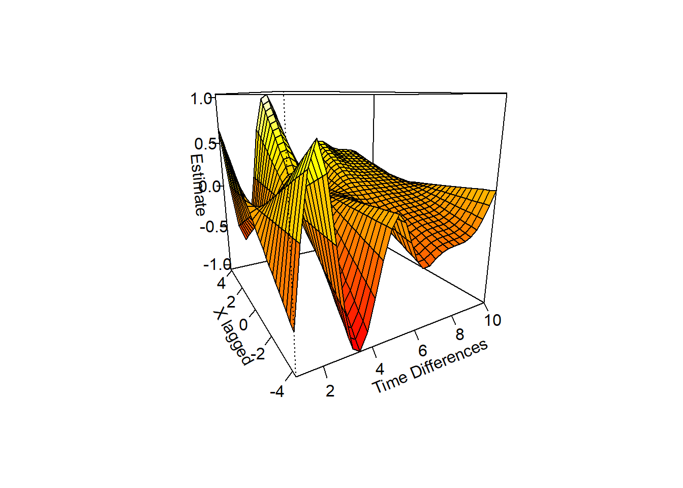
This clearly shows a positive lag at 1, a negative lag at 2, and a positive lag at 3.
Okay, the results of the final state-space model were:
out$OpenMxstage2out$OpenMxout## name matrix row col Estimate Std.Error lbound ubound lboundMet
## 1 XlagonXlag1 s1.A 1 1 0.2360088 0.04461888 NA NA FALSE
## 2 XlagonXlag2 s1.A 1 2 -0.2485319 0.04220480 NA NA FALSE
## 3 XlagonXlag3 s1.A 1 3 0.2835748 0.04300307 NA NA FALSE
## uboundMet tstat pvalue sig
## 1 FALSE 5.289438 1.226928e-07 TRUE
## 2 FALSE -5.888712 3.892167e-09 TRUE
## 3 FALSE 6.594293 4.272871e-11 TRUESo, X predicts significantly itself positively 1 lag later, negatively 2 hours later, and positively again 3 hours later.